Antarctic Animal Tracking Viewer

This document explains the creation of an advanced version of the Marine Mammals Viewer.

Keep in mind, that this is a use case, which means that data managemeint and map service creation remain theoretical but the viewer configuration can be reproduced by yourself using an O2A Portal.

Motivation

You are interested in mammals and considered the Marine Mammals Viewer quite useful. However, you're aware of a more exhaustive data source – the Retrospective Analysis of Antarctic Tracking Data (RAATD) – and would like to increase its accessibility by presenting it in a way similar to the Marine Mammals Viewer. You start reading the docs 🤓.

INFO

For reading and understanding this use case, you neither have to read the docs beforehand nor completely. When following along the viewer configuration part further down the line, specific subsections, that are linked, might turn out useful.

Data Management

INFO

This section is theoretical. Just read and enjoy. Or jump to its end and continue with viewer configuration.

After reading the viewer documentation you find out that your data needs to be hosted as a map service. You start with the Viewer Procedure, contact O2A Support and together you figure out the data flow.

For all RAATD data, the O2A Support and you decide that GeoCSV files – following the O2A GeoCSV specification – are the appropriate choice. Using a project subfolder on AWI's Isilon network storage to exchange the data is agreed upon. You will take care of data pre-processing and will deposit the resulting files in the exchange directory. The O2A Spatial Data Infrastructure (O2A SDI) will check regularly for updates to integrate into the map service automatically.

Data pre-processing is a task for you, as you're the expert on animal tracking data. After downlading the source data (about 80 MB) you're happy to find that they already come as CSV files. You decide to join both files by column event_id and undertake a bunch of processing steps:

• date/time format harmonisation
• augmentation with information on class, DOI and WoRMS URLs
• dropping and/or renaming columns according to the O2A GeoCSV specs

You decide to split the data by class to have two separate datasets – birds and mammals – which you then place on the network drive.

The tool of your trade has been a self-written Python script and you choose to only run it manually, when the source data receive an update.

WARNING

The actual marine mammals dataflow differs from this, as it has been established a decade ago. However, that is a deprecated dataflow.

Map Service

Your data will result in two map service layers: one visualising mammal occurrences, one visualising bird occurrences. From the docs you know that your layers are configured using the dataproduct configuration repository. You learned that symbology and metadata can be updated by yourself using merge requests.

After the O2A support has setup the basic configuration, you send merge requests to

• update title, abstract and keywords in owner.layer.toml,
• add symbology information (*.sld files), and
• structure metadata representation in viewer popups (resources/*.md files)

The following code blocks show excerpts from three changed files: owner.layer.toml, mammals_by_species.sld, and resources/popup.md.

🗎 owner.layer.toml

# [...]

[scar_mammals]

title = "Antarctic Mammal Tracking"
settings.style_default = "mammals_by_species"
settings.style_alternatives = [ "generic" ]
keywords = [ "mammals", "animals", "tracking", "SCAR", ]

# [...]

🗎 mammals_by_species.sld

<!-- [...] -->

<sld:Rule>

  <sld:Title>Crabeater seal</sld:Title>

  <ogc:Filter>
    <ogc:PropertyIsEqualTo>
      <ogc:PropertyName>vernacular_name</ogc:PropertyName>
      <ogc:Literal>Crabeater seal</ogc:Literal>
    </ogc:PropertyIsEqualTo>
  </ogc:Filter>

  <sld:PointSymbolizer>
    <sld:Graphic>
      <sld:Mark>
        <sld:WellKnownName>circle</sld:WellKnownName>
        <sld:Fill>
          <sld:CssParameter name="fill">#00A884</sld:CssParameter>
        </sld:Fill>
        <sld:Stroke>
          <sld:CssParameter name="stroke">#007A5E</sld:CssParameter>
          <sld:CssParameter name="stroke-width">1</sld:CssParameter>
        </sld:Stroke>
      </sld:Mark>
      <sld:Size>6</sld:Size>
    </sld:Graphic>
  </sld:PointSymbolizer>

</sld:Rule>

<!-- [...] -->

🗎 _resources/popup.md

{setTitle(properties.vernacular_name)}

|                 |                                                                |
| --------------- | -------------------------------------------------------------- |
| Occurence Date  | {properties.date}                                              |
| Vernacular Name | {properties.vernacular_name}                                   |
| Scientific Name | {properties.scientific_name} ([WoRMS]({properties.worms_url})) |
| Life Stage      | {properties.life_stage}                                        |
| Sex             | {properties.sex}                                               |
| DOI             | [{properties.doi_url}]({properties.doi_url})                   |

INFO

The details of these files are beyond the scope of this document but their existence is important and will be referred to later.

In the background, SDI automation takes care of these information being processed, resulting in ready-to-use layers. For historical reasons, which will not be elaborated on here, O2A support and you have decided to place these layers in different map services.

Dataproduct	Layer Name	Base + Capabilities URLs
Mammals	mammals_4326	https://maps.awi.de/services/projects/gs/animal_tracking/ows
Birds	birds_4326	https://maps.awi.de/services/projects/gs/animal_tracking/ows

INFO

With these URLs, the theory-only part is over. As these map services and layers actually exist, they can be used by readers to create their own viewer following the steps in the next section.

Viewer Configuration

INFO

This section can be read as a story, or the reader can follow along to recreate the viewer themselves using an O2A Portal like Marine Data.

Now that your Antarctic Animal Tracking data is published as map service layers (see end of Map Service section) you visit Marine Data and log in before you start with a new empty viewer.

From reading the viewer configuration manual you know that viewer creation consists of roughly three different topics: data, filters, and viewer metadata.

As data and filters are interrelated topics you decide to start with the easier task of adding viewer metadata. Afterwards you plan to add your layers and filter widgets.

Viewer Metadata

You enter a title and a description for your project. Then you add all the contributors, who are in charge of the project or respectivley for the viewer curation. Your efforts result in the following sidebar tabs.

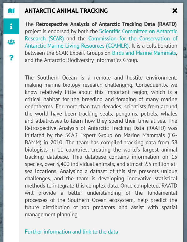
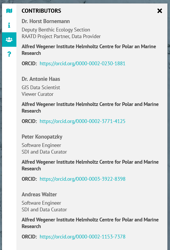
Viewer Metadata. Left: title and description, right: contributors.

Animal Tracking Data

Once you have added the viewer metadata, you proceed to add layers and configure configure filter widgets.

Layer

Using the OGC Importer, you add the Antarctic Mammal Tracking layer.

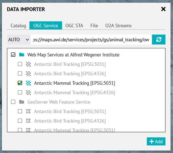
The default style you configured in the back end is fine.

Temporal Filter

Now you add a temporal filter widget and configure it:

• Put date to Column to tell the widget which field/column tu use for temporal filtering.
• The Marine Mammals layer allows you to filter by specific months and years, as well as by time intervals. Therefore you select all listed operators: = , -, >, ≥, <, ≤
• You also choose the multi-slider mode. This enables users to easily switch between comparable points in time.

INFO

To stop users viewing data without knowing its date, you can hide the filter widget's power button: See again the temporal filter configuration part of the creator maunal.

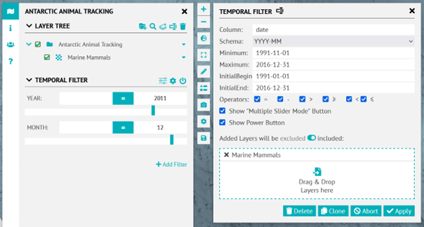
Attribute Filters

As well as the temporal filter, you want to provide more filter options, such as the type of mammal, the sex and age. To do this, add some check-box filters.

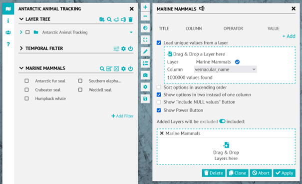
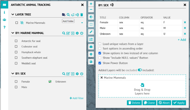
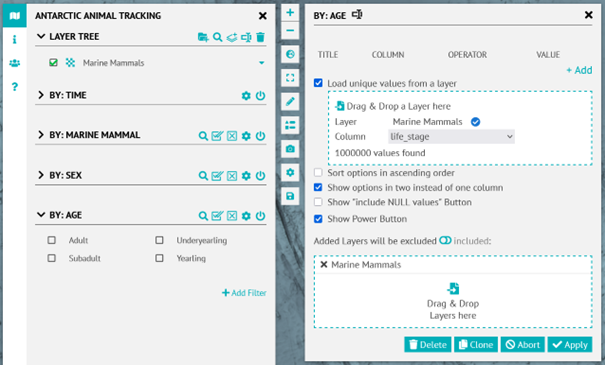
Finally, you have meaningfully changed all the filter names and configured the sidebar as follows:

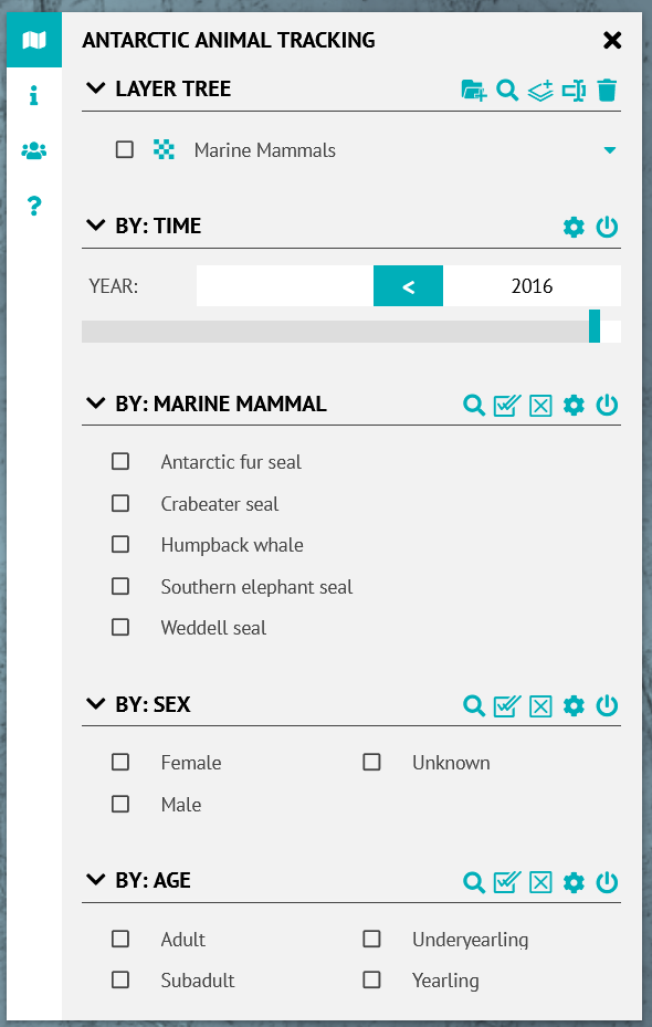
You are happy with both the data visualisation and the filters that can be applied. If you would like to add more data, please follow the Complimentary Data instructions.

Complimentary Data

You also want to add some data from third-party sources to supplement your own data. To do this, you use the data importers Catalog tab. As soon as you type in "Antarctic" in the search line, all data services are listed.

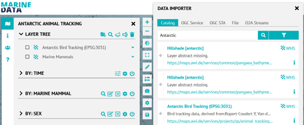
You select Antarctic Bird Tracking (EPSG:3031) and it is automatically listed in the layers tree. You rename it to Birds and add it as a second layer to time filter widget.

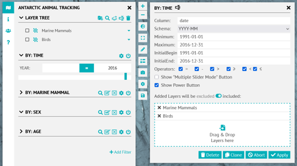
Some of the filters that have already been added, such as the time filter, may be relevant to the birds data. Then you just need to add the layer to the filter. To configure another filter for this layer, such as by bird name, you need to add a new filter and repeat the configuration process.

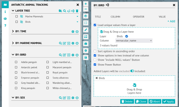
You have now configured the Antarctic Animal Tracking viewer properly, and you are very happy with how your project and data are presented.

Summary

Once the data services are available, configuring the viewer will no longer be the most time-consuming part of the work. The written part is almost complete, starting with the metadata (description, contributors, permissions, etc.).

Adding data and configuring filters will require some preparation time. For example, would you like to focus solely on marine mammals or include more data? If so, you will need to choose a more neutral name for the viewer. 'Antarctic Animal Tracking' instead of 'Marine Mammals Tracking', for instance. The same is true for the filters. Which parameters do you want to focus on, and are these shared by the layers?

However, nothing is set in stone, and once you decide to add something, you can change the names and filters accordingly or simply save it as a new viewer.