Sea Ice Viewer

This document explains the creation of a viewer that is inspired by the Sea Ice Viewer, which has been part of AWI's Sea Ice Portal since the mid-2010s. All steps from motivation to viewer configuration are covered.

Some sections remain theoretical. However, while following the Viewer Configuration section, the reader can recreate the viewer themselves using the Marine Data Portal.

All steps are in line with the according parts of the O2A documentation, especially the Viewer Procedure, and the viewer configuration manual.

This is not a click-by-click manual. The focus is on reasons and decisions. However, there are links to the relevant sections of the viewer configuration manual, helping the reader to recreate the viewer on their own. For the sake of simplicity, some details of the productive viewer are left out and the process is described in an idealised way.

Motivation

You have sea ice concentration (SIC) data, derived from satellite measurements. They are on a daily basis. You used that data to calculate the monthly sea ice median edge (SIME). New data keeps coming!

Now you would like to present these data as time series and make them publicly explorable. To achieve this, you decide to create a Marine Data Viewer and start reading the docs 🤓.

INFO

For reading and understanding this use case, you neither have to read the docs beforehand nor completely. When following along the viewer configuration part further down the line, specific subsections, that are linked, might turn out useful.

Data Management

INFO

This section is theoretical. Just read and enjoy. Or jump to its end and continue with viewer configuration.

After reading the viewer documentation you find out that your data needs to be hosted as a map service. You start with the Viewer Procedure, contact O2A Support and together you figure out the data flow.

For the daily concentration, which is raster data, the O2A Support and you decide that GeoTIFF files – following the O2A GeoTIFF specification – are the best choice. For the monthly median edge, which is vector data, GeoCSV files – following the O2A GeoCSV specification – should do the trick.

Using a project folder on AWI's Isilon network storage to exchange the data is agreed upon. You will deposit the initial files and regularly add new data. The O2A Spatial Data Infrastructure (O2A SDI) will check regularly for new data to integrate into the map services automatically.

INFO

The GeoTIFF and GeoCSV files need to be generated/derived from the source data. How to do and automate this, is beyond the scope of this document. Usually, GDAL is used, either directly or as part of a more high-level library/software. GDAL is a powerful software library for geospatial data processing.

Map Service

Your data will result in two map service layers: one visualising daily sea ice concentration, one visualising the monthly sea ice median edge. From the docs you know that your layers are configured using the dataproduct configuration repository. You learned that symbology and metadata can be updated by yourself using merge requests.

After the O2A support has setup the basic configuration, you send merge requests to

• update title, abstract and keywords in owner.layer.toml,
• add symbology information (*.sld files), and
• structure metadata representation in viewer popups (resources/*.md files)

The following code blocks show excerpts from three changed files: owner.layer.toml, sea_ice_concentration_2.sld, and resources/popup.md.

🗎 owner.layer.toml

# [...]

title = "Sea Ice Concentration (global)"

abstract = 'Sea Ice Concentration (coverage in %). Spatial Resolution: 3.125 km. Temporal Coverage: daily, since 2006. GCOMW1 AMSR2 passive microwave (acknowledgement to JAXA) processed by University of Bremen.'

keywords = [ "sea ice concentration", "satellite imagery", "remote sensing" ]

settings.style_default = "sea_ice_concentration_2"

# [...]

🗎 sea_ice_concentration_2.sld

<!-- [...] -->

<sld:ColorMap>
    <sld:ColorMapEntry color="#f7fbff" label="   0.0 %" opacity="0.0" quantity="0"/>
    <sld:ColorMapEntry color="#deebf7" label="   6.5 %" opacity="0.2" quantity="6.5"/>
    <sld:ColorMapEntry color="#c7dcef" label="  13.0 %" opacity="0.5" quantity="13"/>
    <sld:ColorMapEntry color="#a2cbe2" label="  19.5 %" opacity="0.7" quantity="19.5"/>
    <sld:ColorMapEntry color="#72b2d7" label="  26.0 %" opacity="1.0" quantity="26"/>
    <sld:ColorMapEntry color="#4997c9" label="  32.5 %" opacity="1.0" quantity="32.5"/>
    <sld:ColorMapEntry color="#2878b8" label="  39.0 %" opacity="1.0" quantity="39"/>
    <sld:ColorMapEntry color="#0d57a1" label="  45.0 %" opacity="1.0" quantity="45"/>
    <sld:ColorMapEntry color="#000000" label="  50.0 %" opacity="1.0" quantity="50"/>
    <sld:ColorMapEntry color="#ffffff" label=" 100.0 %" opacity="1.0" quantity="100"/>
</sld:ColorMap>

<!-- [...] -->

🗎 resources/popup.md

|                       |                                        |
|-----------------------|----------------------------------------|
| Sea Ice Concentration | {round(properties.GRAY_INDEX, "3")} %  |
| Sensor URN            | [satellite:gcomw1:amsr2:l2:sic](https://sensor.awi.de/?urn=satellite:gcomw1:amsr2:l2:sic) |

INFO

The details of these files are beyond the scope of this document but their existence is important and will be referred to later.

In the background, SDI automation takes care of these information being processed, resulting in ready-to-use layers. For historical reasons, which will not be elaborated on here, O2A support and you have decided to place these layers in different map services.

Data	Layer Name	Map Service URL
sea ice concentration	gcomw1_amsr2_l2_sic_4326	https://maps.awi.de/services/platforms/satellite/ows
sea ice median edge	sea_ice_median_edge	https://maps.awi.de/services/common/meereisportal/ows

INFO

With these URLs, the theory-only part is over. As these map services and layers actually exist, they can be used by readers to create their own viewer following the steps in the next section.

Viewer Configuration

INFO

This section can either be read as a story or be followed along by the reader to recreate this viewer on their own using an O2A Portal like Marine Data.

Now that your sea ice data is published as map service layers (see end of Map Service section) you visit Marine Data and log in before you start with a new empty viewer.

From reading the viewer configuration manual you know that viewer creation consists of roughly three different topics: data, filters, and viewer metadata.

As data and filters are interrelated topics you decide to start with the easier task of adding viewer metadata. Afterwards you plan to add your layers one by one, each accompanied by a temporal filter widget.

Viewer Metadata

You enter a title and a description for your project. As contributors you add yourself and one of your colleagues who helps with data management. Your efforts result in the following sidebar tabs.

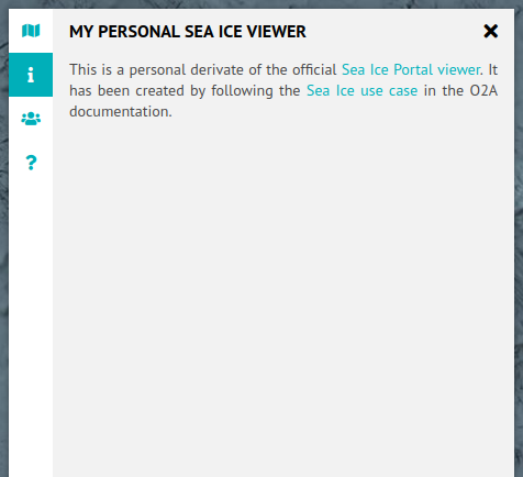
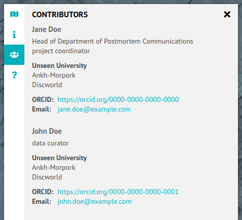
Viewer Metadata. Left: title and description, right: contributors.

Sea Ice Concentration Data

Layer

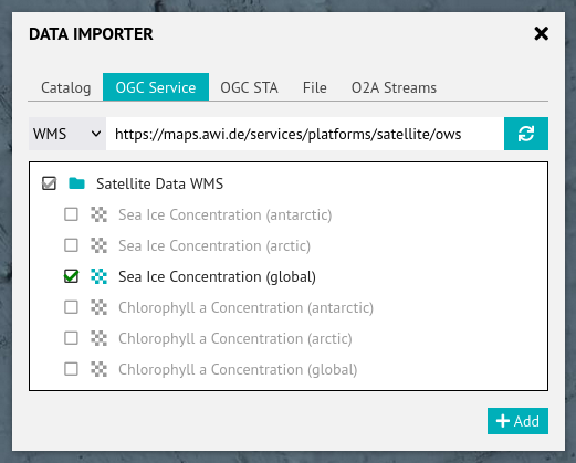
Using the OGC Importer, you add the sea ice concentration layer.

The default style you configured in the back end is fine.

Temporal Filter

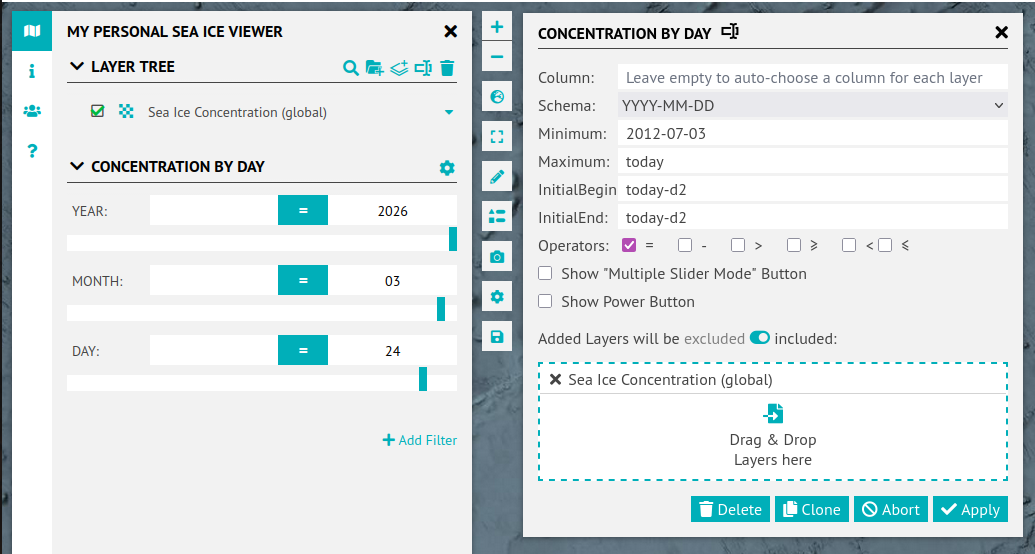
Now you add a temporal filter widget and configure it.

As the concentration layer only supports specific points in time (day) you restrict the temporal filter to the = operator. To prevent users from viewing concentration data without knowing its date, you hide the filter widget's power button. You also choose the multi-slider mode as this enables users to easily switch between comparable points in time.

The value range is configured to dynamically cover a range from the earliest data to the day, users load the viewer. Since you receive your source data and processing also takes some time, you define the day before yesterday as default position for the temporal filter widget slider. This way, you ensure that data is shown when the viewer is loaded.

Next, you restrict the filter widget to the concentration layer and give it a descriptive name. This results in the following configuration.

From the editor manual you learn that to filter your SIC layer, the SIC layer's configuration within the viewer configuration has to be augmented with extra metadata on which attribute to filter. As this has to be done directly in the JSON file that holds the viewer configuration, you decide to just let the O2A support implement this for you.

augmented layer configuration

  "layers": {
    "0830d4e9": {
      "catalogId": "zptcihL2",
      "queryParams": {
        "styles": "sea_ice_concentration_2"
      },
      "attributeFields": {
        "date_time": {
          "type": "dateTime"
        }
      },
      "active": true
    }
  },

added excerpt

"attributeFields": {
  "date_time": {
    "type": "dateTime"
  }
},

Sea Ice Median Edge Data

Layer

Using the OGC Importer, you add the sea ice median edge layer. From the available styles you choose the one with turquoise lines.

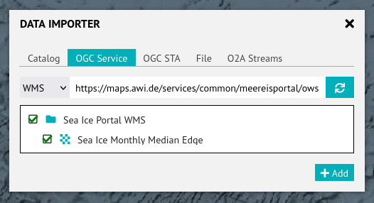
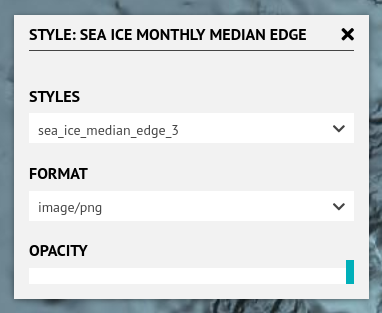
Adding the median edge layer. Left: OGC importer, right: style configuration.

Afterwards, you ensure that the median edge layer is listed above the concentration layer (see user manual). Otherwise, due to its continuous character, the concentration data might overlap and hide the discrete lines of the median edge data, whereas discrete lines ontop continuous raster data work well.

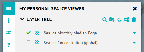
Re-arranged layer tree with core data layers: median edge (vector) ontop concentration (raster).

Temporal Filter

To be able to compare concentration data with median edge data from other points in time you add another temporal filter widget.

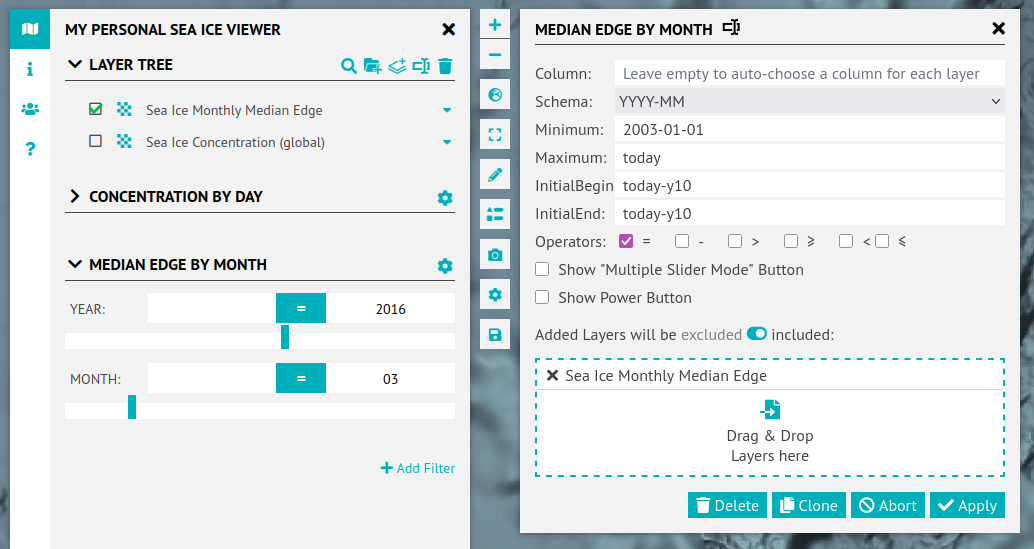
As you do want users to filter for median edge data of specific months, you restrict the temporal filter to the = operator. To prevent users from viewing all median edge data at the same time, you hide the filter widget's power button. You also choose the multi-slider mode as this enables users to easily switch between comparable points in time.

The value range is configured to dynamically cover a range from the earliest data to the month before the month, users load the viewer. To have a meaningful comparision as default, you choose to display the median edge data from ten years ago.

Last but not least, you restrict the filter widget to the median edge layer and give it a descriptive name. This results in the following configuration.

Complementary Data

Now that you're done making your sea ice data available and explorable to the public, you decide to add complementary data. Browsing the catalog find two interesting layers for your viewer. One that offers near real-time positions of buoys drifting in the Arctic and Antarctic Ocean, measuring e.g. surface temperature; and one that offers current tracklines of research vessels, including the famous Polarstern.

Buoys

Using the Layer Catalog, you add the layer with buoys position data. The default style seems fine.

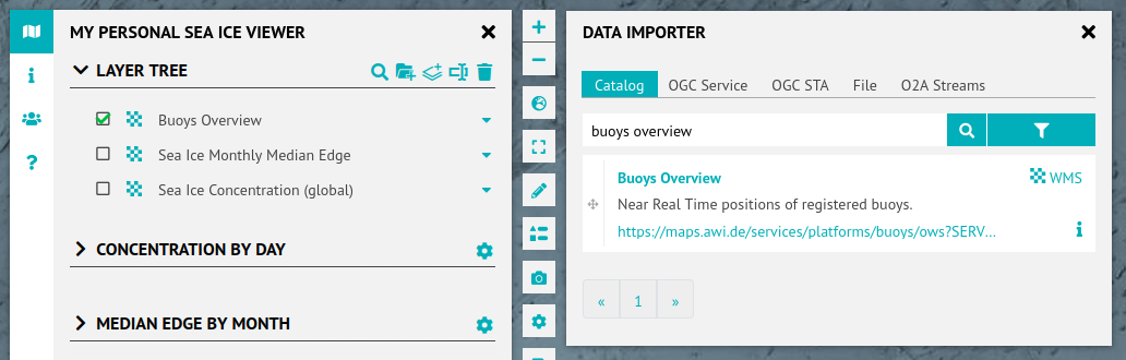
To prevent the layer from loading millions of historic positions you decide to couple it with the time filter widget filtering the sea ice concentration by day. As there are different types of buoys, you add an attribute filter widget with checkboxes to filter buoys by type.

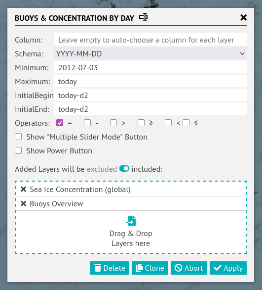
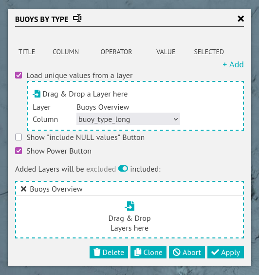
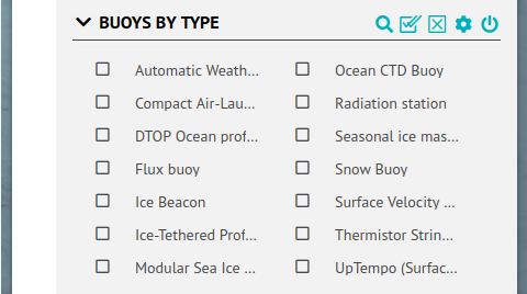
Buoys Filters. Left: updated time filter settings, middle: buoy type filter settings, right: buoy type filter widget.

Polarstern Track

Using the Layer Catalog, you add a layer with current tracklines of research platforms.

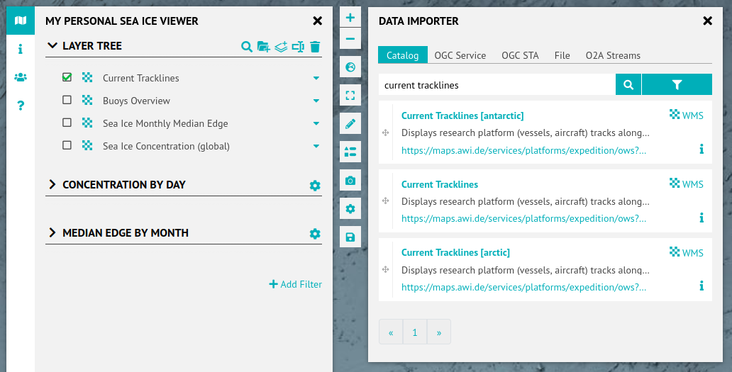
Checking the available styles you discover one that only shows the current Polarstern track, tracklines_polarstern, and decide to use that style. As it only shows the current track anyway, there's no need to apply any time filter.

Summary

You created two WMS layers from your sea ice data in collaboration with the O2A support. Afterwards you created a new viewer, adding these layers and configuring different time filter widgets to make the data explorable in a useful way. Finally, you added complementary data that has been available previously and combined it with an attribute filter widget.